41 pivot table row labels format
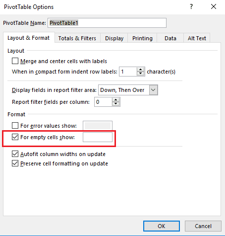
Accessible Rich Internet Applications (WAI-ARIA) 1.1 - W3 For example, a scripting library can determine the labels for the tree items in a tree view, but would need to prompt the author to label the entire tree. To help authors visualize a logical accessibility structure, an authoring environment might provide an outline view of a web resource based on the WAI-ARIA markup. Formatting Tips for Pivot Tables - Goodly Right Click on the Pivot and go to Pivot Table Options Under Layout & Format Tab --> For empty cells show: "NIL" (you can customize this) Tip #11 Custom Sorting of Row / Column values This happens a lot. The default sorting order of row or column (text) labels is A-Z or Z-A. Now there are 2 ways to sort the values in a custom order
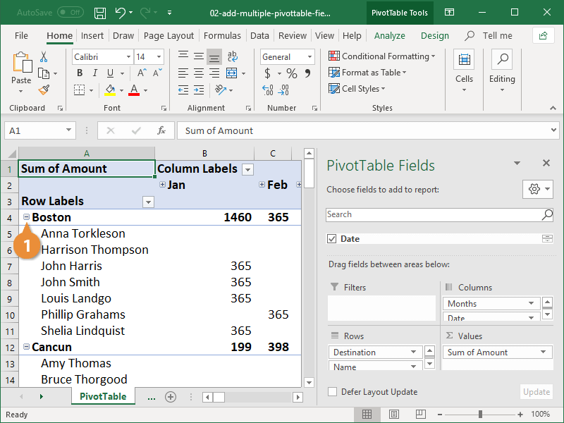
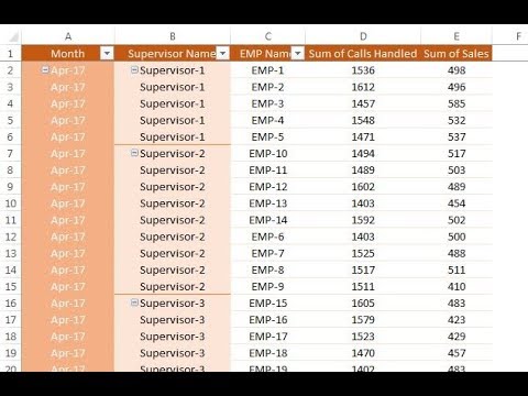
Change Pivot Table Layout using VBA - Access-Excel.Tips Even worse, the column label "Department" and "Empl ID" are gone. I personally hate this layout because it does not use the actual column name, instead it uses "Row Labels", "Column Labels". Since "Row Labels" refer to both Department and Empl ID as they display in one column, it uses a generic name "Row Labels".
Pivot table row labels format
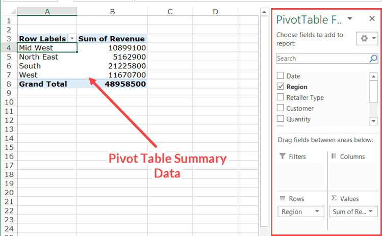
Design the layout and format of a PivotTable To change the format of the PivotTable, you can apply a predefined style, banded rows, and conditional formatting. Windows Web Mac Changing the layout form of a PivotTable Change a PivotTable to compact, outline, or tabular form Change the way item labels are displayed in a layout form Change the field arrangement in a PivotTable Excel: How to Sort Pivot Table by Date - Statology Before creating a pivot table for this data, click on one of the cells in the Date column and make sure that Excel recognizes the cell as a Date format: Next, we can highlight the cell range A1:B10, then click the Insert tab along the top ribbon, then click PivotTable, and insert the following pivot table to summarize the total sales for each ... Overwrite pivot table conditional format based on row label As far as I know, using the one rule in the Conditional formatting, we can only format the cells with one color if the condition is true and if the same condition is false, the formatting of the cell will be blank and if both conditions are true, the formatting of cell depends on the highest ranking/priority of the rules in Conditional formatting.
Pivot table row labels format. How to Format the Values of Numbers in a Pivot Table Click the Insert tab, then Pivot Table. This will launch the Create PivotTable dialog box. Figure 3. Inserting a Pivot Table. Step 3. In the Create PivotTable dialog box, tick Existing Worksheet. Click the bar for Location and then click cell H2. This will position the pivot table in the existing worksheet, at cell H2. Figure 4. How to format numbers in a pivot table - Exceljet The first way is to click the field drop-down menu, and choose Value field settings. Then, in the Value Field Settings dialog box, click the Number Format option and apply the format you like. The second way to set number formatting is to right-click on a value directly in the pivot table, and select Value field settings from the menu. Repeat item labels in a PivotTable - support.microsoft.com Right-click the row or column label you want to repeat, and click Field Settings. Click the Layout & Print tab, and check the Repeat item labels box. Make sure Show item labels in tabular form is selected. Notes: When you edit any of the repeated labels, the changes you make are applied to all other cells with the same label. How to Create a Pivot Table in Excel - Spreadsheeto Using Pivot Table Fields. A Pivot Table ‘field’ is referred to by its header in the source data (e.g. ‘Location’) and contains the data found in that column (e.g. San Francisco). By separating data into their respective ‘fields’ for use in a Pivot Table, Excel enables its user to:
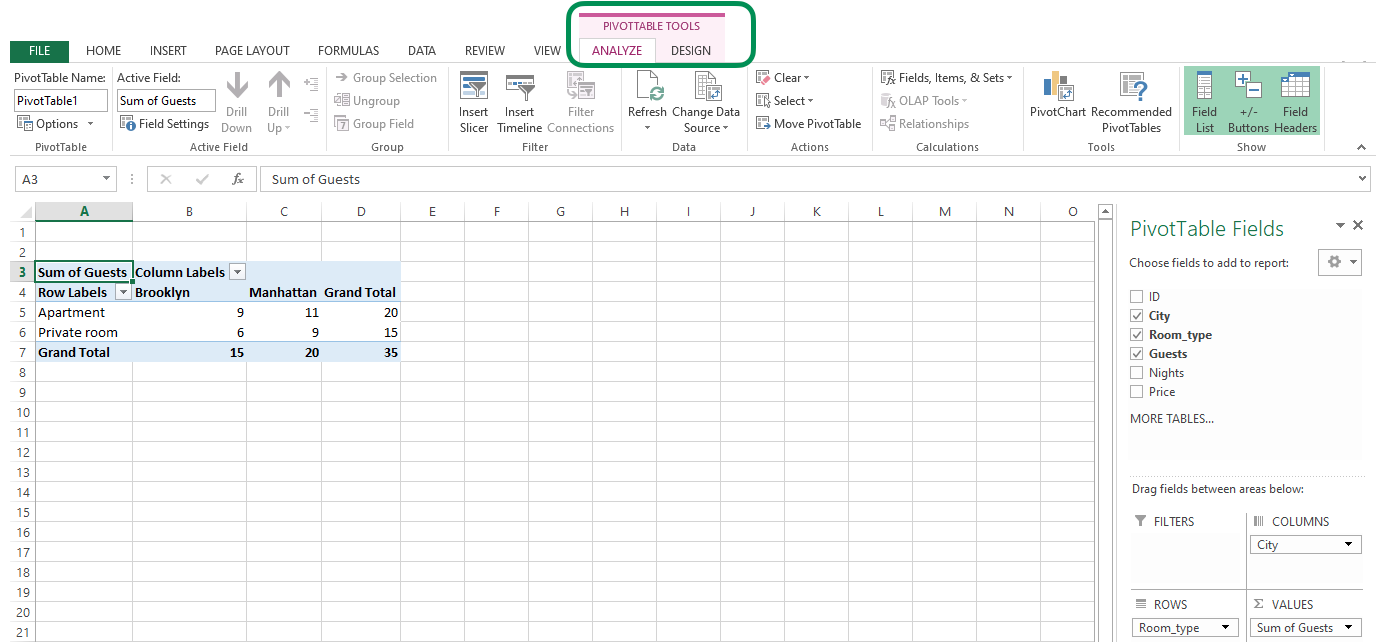
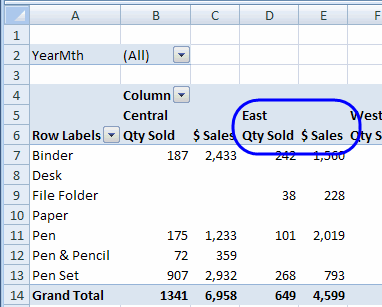
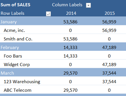
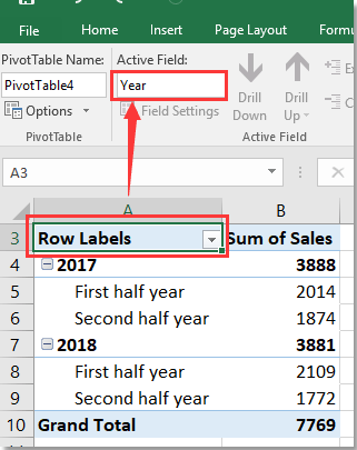
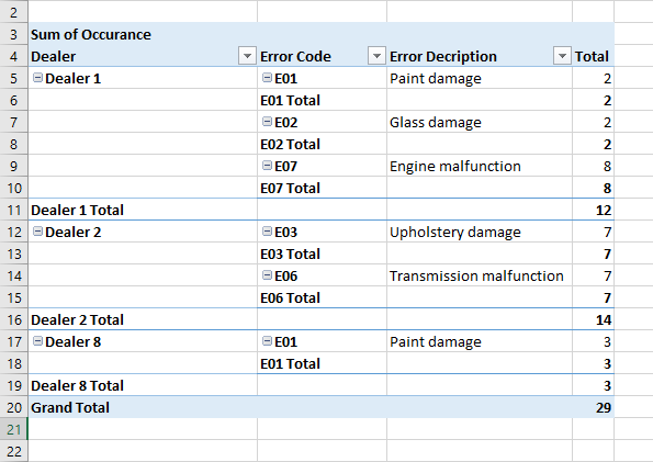
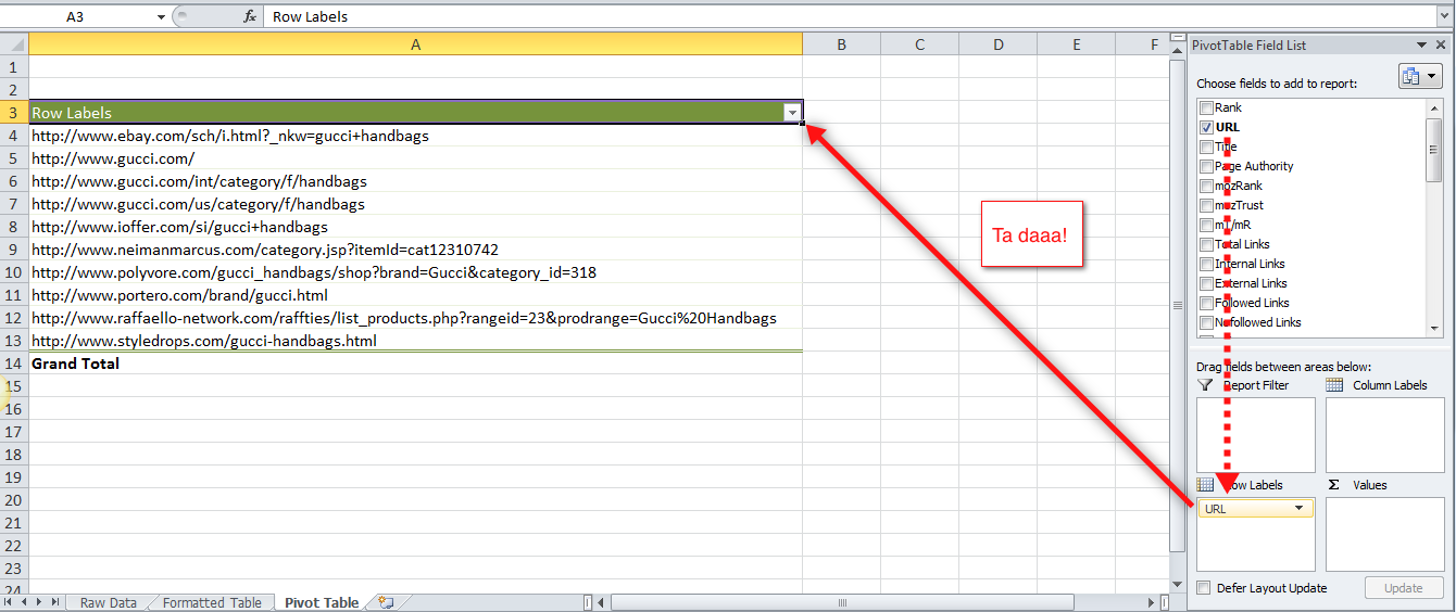
Conditional Formatting on Pivot Table row labels In srcFromPowerPivot sheet cell A is from powerpivot under row label comparing the dates in cell C (3 dates) and the condtional formatting doesnt work. In cell J it worked cos I dragged under value instead of row label. In the srcFromWorksheet it worked even though it is under rowlabel. Sheet3 is just a copy of powerpivot data. Pivot Table Row Label Date Formating | MrExcel Message Board #1 I have my pivot table set up One of the row labels is a date field, however I cannot get it to stay in the date format I wish, it keeps defaulting to dd/mm/yyyy The source column is set to format dd mmm yyyy. Every time I try something to change to date format in the pivot table, it defaults back again. any pointers or help out there. Pivot table row labels side by side - Excel Tutorial - OfficeTuts Excel You can copy the following table and paste it into your worksheet as Match Destination Formatting. Now, let's create a pivot table ( Insert >> Tables >> Pivot Table) and check all the values in Pivot Table Fields. Fields should look like this. Right-click inside a pivot table and choose PivotTable Options…. Check data as shown on the image below. How to rename group or row labels in Excel PivotTable? - ExtendOffice To rename Row Labels, you need to go to the Active Field textbox. 1. Click at the PivotTable, then click Analyze tab and go to the Active Field textbox. 2. Now in the Active Field textbox, the active field name is displayed, you can change it in the textbox.
PivotTable Indentations? Use the Select option in the PivotTable Tools ribbon tab to select the labels (Select "Entire PivotTable" then immediately select "Labels" from the same drop-down (very counter intuitive)). Then got to Home tab on the ribbon and use "Clear" to clear formats. Indents should be restored to whatever value is set in the PivotTable options. Excel Pivot Table - Format Numbers in Rows To format rows or columns in a PT, hover the mouse at the top of the column or beginning of the row until a black arrow appears, click to highlight the row/column and format as usual. For Display labels from next field in same column, uncheck this, follow above procedure, then recheck. Paula Scharf 50 Things You Can Do With Excel Pivot Table | MyExcelOnline Jul 18, 2017 · STEP 1: Click in your data and go to Insert > Pivot Table. STEP 2: This will bring up the Create Pivot Table dialogue box and it will automatically select your data`s range or table. In the Choose where you want the PivotTable report to be placed, you can either choose a New Worksheet or an Existing Worksheet. python - How can I pivot a dataframe? - Stack Overflow Nov 07, 2017 · crosstab() calls pivot_table(), i.e., crosstab = pivot_table. Specifically, it builds a DataFrame out of the passed arrays of values, filters it by the common indices and calls pivot_table(). It's more limited than pivot_table() because it only allows a one-dimensional array-like as values, unlike pivot_table() that can have multiple columns as ...
Add Multiple Columns to a Pivot Table | CustomGuide
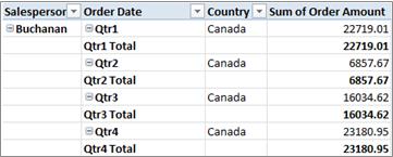
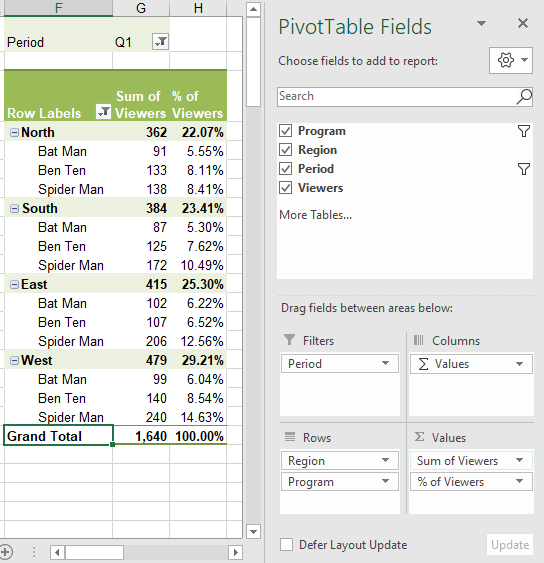
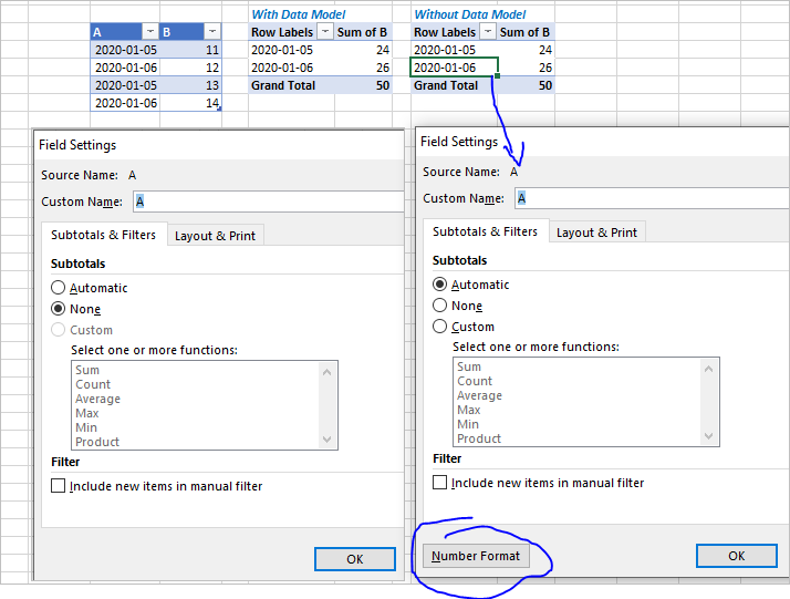
How to Change Date Format in Pivot Table in Excel - ExcelDemy Firstly, click on the Group Selection option in the PivotTable Analyze tab while keeping the cursor over a cell of the Order Date (Row Labels). Secondly, you'll get the following dialog box namely Grouping. And choose Years from the options. Finally, you'll get the sum of sales based on the years instead of the dates. 3.2.
The Pivot table tools ribbon in Excel
Formatting Pivot Table Row Labels by Level | MrExcel Message Board hover your cursor over the top line of one of the SubTotals of the Level that you want to format until you get a downward pointing, then left click - that should highlight all the cells at that level right click while hovering over one of the selected cells to format it OR hit Ctrl+F1

Microsoft Excel – showing field names as headings rather than ...
Automatic Row And Column Pivot Table Labels - How To Excel At Excel Select the data set you want to use for your table The first thing to do is put your cursor somewhere in your data list Select the Insert Tab Hit Pivot Table icon Next select Pivot Table option Select a table or range option Select to put your Table on a New Worksheet or on the current one, for this tutorial select the first option Click Ok
Design the layout and format of a PivotTable
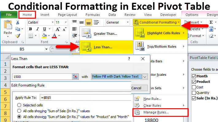
Conditional Formatting in Pivot Table - WallStreetMojo To apply conditional formatting in the pivot table, first, we must select the column to format. In this example, select "Grand Total Column.". Then, in the "Home" Tab in the "Styles" section, click on "Conditional Formatting.". Consequently, a dialog box pops up. Then, we need to click on "New Rule.". As a result, another ...
My Biggest Pivot Table Annoyance (And How To Fix It ...
Data Labels in Excel Pivot Chart (Detailed Analysis) Add a Pivot Chart from the PivotTable Analyze tab. Then press on the Plus right next to the Chart. Next open Format Data Labels by pressing the More options in the Data Labels. Then on the side panel, click on the Value From Cells. Next, in the dialog box, Select D5:D11, and click OK.
Quick Pivot Table Tip-1: Tabular Form with Repeat All Item Labels
PivotTable.RowFields property (Excel) | Microsoft Learn This example adds the PivotTable report's row field names to a list on a new worksheet. VB Set nwSheet = Worksheets.Add nwSheet.Activate Set pvtTable = Worksheets ("Sheet2").Range ("A1").PivotTable rw = 0 For Each pvtField In pvtTable.RowFields rw = rw + 1 nwSheet.Cells (rw, 1).Value = pvtField.Name Next pvtField Support and feedback
Centre Column Headings in Excel Pivot Table | Excel Pivot Tables
Format Pivot Table Labels Based on Date Range In the pivot table, remove any filters that have been applied - all the rows need to be visible before you apply the conditional formatting. Select all the dates in the Row Labels that you want to format. On the Ribbon, click the Home tab, and then in the Styles group, click Conditional Formatting.

Pivot table row labels side by side – Excel Tutorial
Pivot Table Row Labels for date values - Microsoft Community Created on August 1, 2017 Pivot Table Row Labels for date values I need my row labels to be the actual value in the field, which happens to be a date field. So, I have several records of the same date (date format) and when I create the Pivot Table, the row label is formatted with tree/expandable options showing the year, Qtr, month.
How to make row labels on same line in pivot table?
101 Advanced Pivot Table Tips And Tricks You Need To Know Apr 25, 2022 · After creating your pivot table you can delete the source data if you want to reduce the workbook file size. You can delete your source data by deleting the sheet it’s contained on. Right click on the sheet tab and select Delete from the menu. Your pivot table contains a cache of the data so it will continue to work as normal.
Design the layout and format of a PivotTable
Pivot Table Row Labels In the Same Line - Beat Excel! Learn how to arrange pivot table roow labels in the same line. Put multiple lables side by side into the same line. ... It is a common issue for users to place multiple pivot table row labels in the same line. ... bar chart Basics column chart Combined Charts comment condition conditional formatting data analysis data validation data ...
Excel Pivot Tables Explained • My Online Training Hub
Pivot Table Formatting - Excel Champs Click anywhere on the PivotTable to activate the design tab. Now, click on the small drop-down arrow in the designs to scroll to the end. Here click on the "New PivotTable Style". Now, a pop-up window will open "New PivotTable Style". Rename the PivotTable in the "Name Field". Select an element to format and click on the "Format ...
How to Insert a Blank Row in Excel Pivot Table | MyExcelOnline
Excel Pivot Table Subtotals Examples Videos Workbooks Oct 10, 2022 · In a new pivot table, when you add fields to the Row Labels area, subtotals are automatically shown at the top of each group of items, for the outer fields. You canmove the subtota ls to the bottom of the group, if you prefer. To move the subtotals, follow these steps. Select a cell in the pivot table, and on the Ribbon, click the Design tab.
How to Delete a Pivot Table in Excel (Easy Step-by-Step Guide)
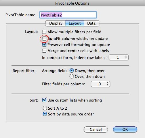
How to make row labels on same line in pivot table? - ExtendOffice Make row labels on same line with PivotTable Options You can also go to the PivotTable Options dialog box to set an option to finish this operation. 1. Click any one cell in the pivot table, and right click to choose PivotTable Options, see screenshot: 2.
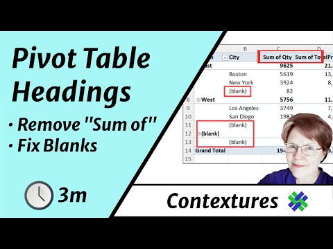
Change Pivot Table Sum of Headings and Blank Labels
How to Create a Pivot Table in Excel: A Step-by-Step Tutorial Dec 31, 2021 · How to Create a Pivot Table. Enter your data into a range of rows and columns. Sort your data by a specific attribute. Highlight your cells to create your pivot table. Drag and drop a field into the "Row Labels" area. Drag and drop a field into the "Values" area. Fine-tune your calculations.
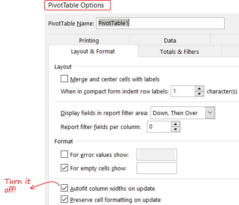
Formatting Tips for Pivot Tables - Goodly
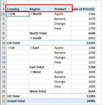
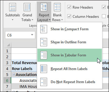
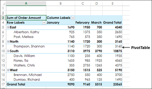
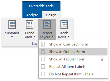
Pivot table row labels in separate columns • AuditExcel.co.za Our preference is rather that the pivot tables are shown in tabular form (all columns separated and next to each other). You can do this by changing the report format. So when you click in the Pivot Table and click on the DESIGN tab one of the options is the Report Layout. Click on this and change it to Tabular form.

Pivot Table Row Labels In the Same Line - Beat Excel!
Excel Pivot table grouping Row Labels that are Percentages Here is my data (apologies for poor formatting, maybe that should have been my first question!): Customer Percentage Increase 1 2% 2 12% 3 -50% 4 87% 5 -20% 6 -1% 7 123% 8 -98% 9 10% 10 13% I created a pivot table in Excel with Percentage Increase as the Row Labels and Count of Customer as the value.
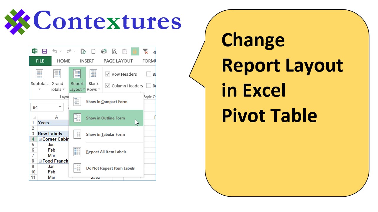
Change Excel Pivot Table Report Layout
How to Format Excel Pivot Table - Contextures Excel Tips Select a cell in any pivot table. On the Ribbon, under the PivotTable Tools tab, click the Design tab. In the PivotTable Style options gallery, right-click on the style that you want to set as the default. In the context menu, click on Set As Default. NOTE: The default PivotTable style selection is for the active workbook only.

How to Format Excel Pivot Table
Overwrite pivot table conditional format based on row label As far as I know, using the one rule in the Conditional formatting, we can only format the cells with one color if the condition is true and if the same condition is false, the formatting of the cell will be blank and if both conditions are true, the formatting of cell depends on the highest ranking/priority of the rules in Conditional formatting.

Excel Tips: Repeat Row Labels in Excel 2007
Excel: How to Sort Pivot Table by Date - Statology Before creating a pivot table for this data, click on one of the cells in the Date column and make sure that Excel recognizes the cell as a Date format: Next, we can highlight the cell range A1:B10, then click the Insert tab along the top ribbon, then click PivotTable, and insert the following pivot table to summarize the total sales for each ...
Making Report Layout Changes | Customizing a Pivot Table in ...
Design the layout and format of a PivotTable To change the format of the PivotTable, you can apply a predefined style, banded rows, and conditional formatting. Windows Web Mac Changing the layout form of a PivotTable Change a PivotTable to compact, outline, or tabular form Change the way item labels are displayed in a layout form Change the field arrangement in a PivotTable
How To Remove (blank) Values in Your Excel Pivot Table - MPUG

Pivot table row labels side by side – Excel Tutorial

How to Format Excel Pivot Table

Pivot table row labels in separate columns • AuditExcel.co.za

How to Format Excel Pivot Table
How to rename group or row labels in Excel PivotTable?
Excel Pivot Tables - Sorting Data

Repeat all item labels in Pivot Table (aka Fill in the blanks ...
Pivot table row labels side by side – Excel Tutorial
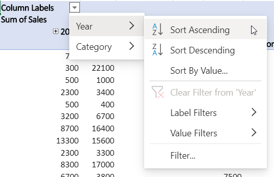
Pivot Table Sort in Excel | How to Sort Pivot Table Columns ...
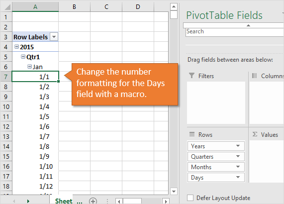
How to Change Date Formatting for Grouped Pivot Table Fields ...
Conditional Formatting in Pivot Table (Example) | How To Apply?
Pivot table row labels side by side – Excel Tutorial
changing Date format in a pivot table - Microsoft Community Hub

How to Format Pivot Tables in Google Sheets - Lido.app
Change the PivotTable Layout | EarthCape Documentation

Repeat item labels in a PivotTable
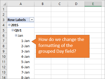
How to Change Date Formatting for Grouped Pivot Table Fields ...

Use Excel PivotTables to quickly analyze grades - Extra Credit
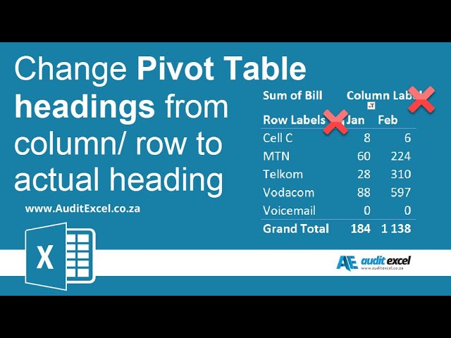
Pivot Table headings that say column/ row instead of actual ...
How To Manage Big Data With Pivot Tables
Post a Comment for "41 pivot table row labels format"