39 excel bar graph labels

How to Add Two Data Labels in Excel Chart (with Easy Steps) 4 Quick Steps to Add Two Data Labels in Excel Chart. Step 1: Create a Chart to Represent Data. Step 2: Add 1st Data Label in Excel Chart. Step 3: Apply 2nd Data Label in Excel Chart. Step 4: Format Data Labels to Show Two Data Labels. Things to Remember. How to Add Axis Labels in Excel Charts - Step-by-Step (2022) How to add axis titles 1. Left-click the Excel chart. 2. Click the plus button in the upper right corner of the chart. 3. Click Axis Titles to put a checkmark in the axis title checkbox. This will display axis titles. 4. Click the added axis title text box to write your axis label.

How to Change Excel Chart Data Labels to Custom Values? At this point excel will select only one data label. Go to Formula bar, press = and point to the cell where the data label for that chart data point is defined. Repeat the process for all other data labels, one after another. See the screencast. Points to note: This approach works for one data label at a time.

Excel bar graph labels

Bar Graph in Excel — All 4 Types Explained Easily To create a simple bar graph, follow these steps: Get your Data ready. Make sure it has one categorical variable and one quantitative secondary variable. In my example from Sheet1, I have the time duration of 6 tasks. Select your Data with headers. Locate and click on the 2-D Clustered Bars option under the Charts group in the Insert Tab. How to Create Bar Chart in Excel? - EDUCBA Step 1: Select the data > Go to Insert > Bar Chart > Cone Chart. Step 2: Click on the CONE chart, and it will insert the basic chart for you. Step 3: Now, we need to modify the chart by changing its default settings. Remove gridlines of the above Chart. Change the chart title to Sales by month. How to Make a Bar Chart in Excel - Smartsheet 25 Jan 2018 — Data labels show the value associated with the bars in the chart. This information can be useful if the values are close in range. To add data ...

Excel bar graph labels. How to Make a Bar Chart in Microsoft Excel Adding and Editing Axis Labels To add axis labels to your bar chart, select your chart and click the green "Chart Elements" icon (the "+" icon). From the "Chart Elements" menu, enable the "Axis Titles" checkbox. Axis labels should appear for both the x axis (at the bottom) and the y axis (on the left). These will appear as text boxes. How to Add Percentages to Excel Bar Chart If we would like to add percentages to our bar chart, we would need to have percentages in the table in the first place. We will create a column right to the column points in which we would divide the points of each player with the total points of all players. We will select range A1:C8 and go to Insert >> Charts >> 2-D Column >> Stacked Column: 2 data labels per bar? - Microsoft Community If people want to see patterns in the data and quickly assimilate this without having to compute things, then a simple, uncluttered chart is ideal. So if you are creating a report for a mixed audience, maybe you need both. But adding lots of labels all over your chart is giving nobody the best result. How to Add Total Data Labels to the Excel Stacked Bar Chart Step 1: Create a sum of your stacked components and add it as an additional data series (this will distort your graph initially) Step 2: Right click the new data series and select "Change series Chart Type…" Step 3: Choose one of the simple line charts as your new Chart Type Step 4: Right click your new line chart and select "Add Data Labels"

How to rotate axis labels in chart in Excel? - ExtendOffice Rotate axis labels in Excel 2007/2010 1. Right click at the axis you want to rotate its labels, select Format Axis from the context menu. See screenshot: 2. In the Format Axis dialog, click Alignment tab and go to the Text Layout section to select the direction you need from the list box of Text direction. See screenshot: 3. How to place labels underneath bar chart - Microsoft Community The names are appearing below the chart axis, that is on value 0.0%. They are on the correct place. If you want them to appear at the bottom of your chart, just select the axis and on the "Format axis" dialog box, on the "Axis options" tab, on the "Axis labels:" option, select "Low". jpgpinto jpgpinto How to Add Total Values to Stacked Bar Chart in Excel Step 4: Add Total Values. Next, right click on the yellow line and click Add Data Labels. Next, double click on any of the labels. In the new panel that appears, check the button next to Above for the Label Position: Next, double click on the yellow line in the chart. In the new panel that appears, check the button next to No line: Text Labels on a Horizontal Bar Chart in Excel - Peltier Tech On the Excel 2007 Chart Tools > Layout tab, click Axes, then Secondary Horizontal Axis, then Show Left to Right Axis. Now the chart has four axes. We want the Rating labels at the bottom of the chart, and we'll place the numerical axis at the top before we hide it. In turn, select the left and right vertical axes.

Bar Chart in Excel | Examples to Create 3 Types of Bar Charts This example illustrates creating a 3D bar chart in Excel in simple steps. Step 1: First, we must enter the data into the Excel sheets in the table format, as shown in the figure. Step 2: We will now select the whole table by clicking and dragging or placing the cursor anywhere in the table and pressing "CTRL+A" to choose the table completely. Histogram with Actual Bin Labels Between Bars - Peltier Tech Select the added series (select the visible series and press the up arrow key, or use one of the chart element picker dropdowns on the ribbon or right click menu), then click the menu key between the Alt and Ctrl keys to the right of the Space bar. This pops up the right click menu. Select Change Series Chart Type, and select one of the Line types. How to Create a Bar Chart With Labels Inside Bars in Excel 1. Highlight the range A5:B16 and then, on the Insert tab, in the Charts group, click Insert Column or Bar Chart > Clustered Bar. The chart should look like this: 2. Next, lets do some cleaning. Delete the vertical gridlines, the horizontal value axis and the vertical category axis. 3. Excel charts: add title, customize chart axis, legend and data labels Select the chart and go to the Chart Tools tabs ( Design and Format) on the Excel ribbon. Right-click the chart element you would like to customize, and choose the corresponding item from the context menu. Use the chart customization buttons that appear in the top right corner of your Excel graph when you click on it.

microsoft excel - How can I create a bar-chart which has multiple bars for each label in MS ...

How to add data labels from different column in an Excel chart? Right click the data series in the chart, and select Add Data Labels > Add Data Labels from the context menu to add data labels. 2. Click any data label to select all data labels, and then click the specified data label to select it only in the chart. 3.

Line Chart in Excel - Easy Excel Tutorial

How do I make excel label every bar in a bar chart? - Super User Insert->Pivot Chart Click Clustered Column Right-click on graph, select Format Axis set specify unit interval to 1 Excel now just labels every 2nd bar, even though it would easily fit (I have about 150 bars) with the given label font size. Even though I have selected 1, it has the same text density as if I set specify unit interval to 2.

How to Create a Bar Chart With Labels Above Bars in Excel

How to Use Cell Values for Excel Chart Labels Select the chart, choose the "Chart Elements" option, click the "Data Labels" arrow, and then "More Options." Uncheck the "Value" box and check the "Value From Cells" box. Select cells C2:C6 to use for the data label range and then click the "OK" button. The values from these cells are now used for the chart data labels.

How to Create a Bar Chart With Labels Above Bars in Excel

Add or remove data labels in a chart - support.microsoft.com In the upper right corner, next to the chart, click Add Chart Element > Data Labels. To change the location, click the arrow, and choose an option. If you want to show your data label inside a text bubble shape, click Data Callout. To make data labels easier to read, you can move them inside the data points or even outside of the chart.

How to Create a Bar Chart With Labels Above Bars in Excel

Grouped Bar Chart in Excel - How to Create? (10 Steps) Step 1: Select the chart. With the selection, the Design and Format tabs appear on the Excel ribbon. In the Design tab, choose "change chart type.". Step 2: The "change chart type" window opens, as shown in the following image. Step 3: In the "all charts" tab, click on "bar.".

How can I hide 0% value in data labels in an Excel Bar Chart - Super User

How to Make a Bar Graph in Excel: 9 Steps (with Pictures) If you want to create a graph from pre-existing data, instead double-click the Excel document that contains the data to open it and proceed to the next section. 2 Add labels for the graph's X- and Y-axes. To do so, click the A1 cell (X-axis) and type in a label, then do the same for the B1 cell (Y-axis).

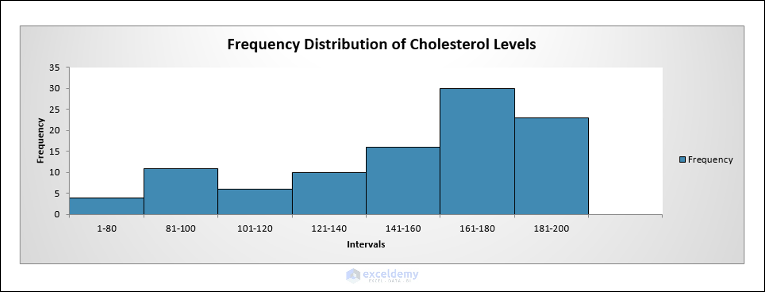
Bar Graph vs Histogram - Difference Between Bar Graph and Histogram!

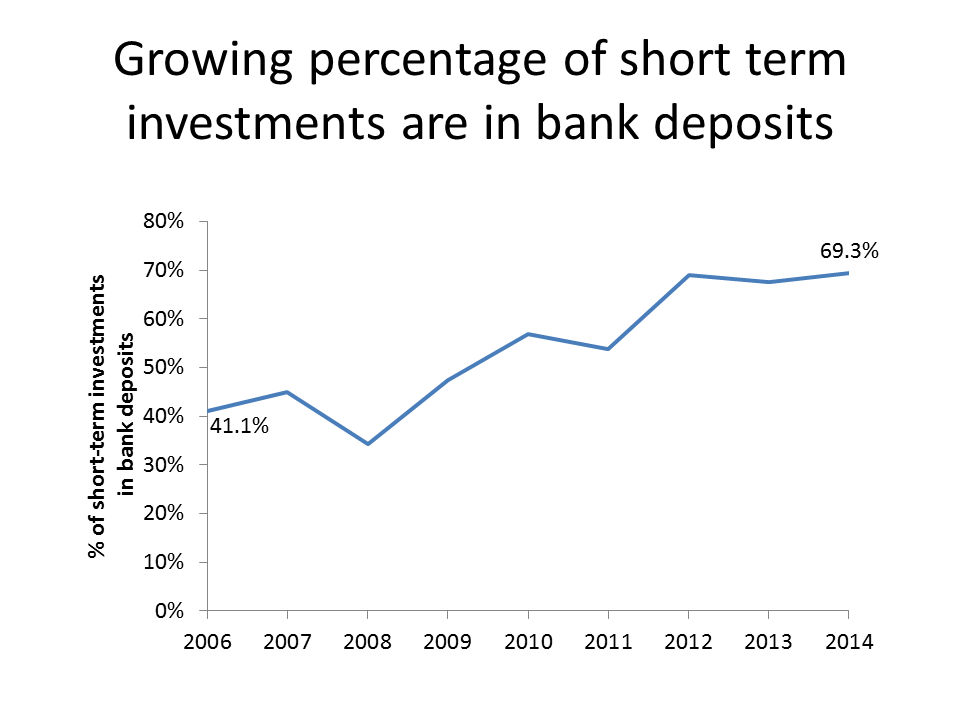
How to label graphs in Excel | Think Outside The Slide If the values are needed, then you will want to use data labels. I suggest placing them inside the end of the column or bar, or just outside the column or bar. This example shows a column graph with data labels only. Example 1 If the message is more related to the ranking of the values, then you can use an axis.

How to label graphs in Excel | Think Outside The Slide

How to Insert Axis Labels In An Excel Chart | Excelchat We will again click on the chart to turn on the Chart Design tab. We will go to Chart Design and select Add Chart Element. Figure 6 - Insert axis labels in Excel. In the drop-down menu, we will click on Axis Titles, and subsequently, select Primary vertical. Figure 7 - Edit vertical axis labels in Excel. Now, we can enter the name we want ...

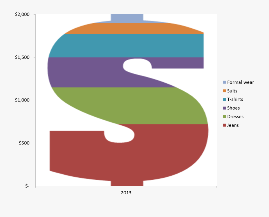
Graph Clipart Secondary Data - Dollar Sign Chart Excel , Free Transparent Clipart - ClipartKey

How to Create a Bar Chart With Labels Above Bars in Excel In the chart, right-click the Series "Dummy" Data Labels and then, on the short-cut menu, click Format Data Labels. 15. In the Format Data Labels pane, under Label Options selected, set the Label Position to Inside End. 16. Next, while the labels are still selected, click on Text Options, and then click on the Textbox icon. 17.

How to Create a Bar Chart With Labels Above Bars in Excel

Edit titles or data labels in a chart - support.microsoft.com Right-click the data label, and then click Format Data Label or Format Data Labels. Click Label Options if it's not selected, and then select the Reset Label Text check box. Top of Page Reestablish a link to data on the worksheet On a chart, click the label that you want to link to a corresponding worksheet cell.

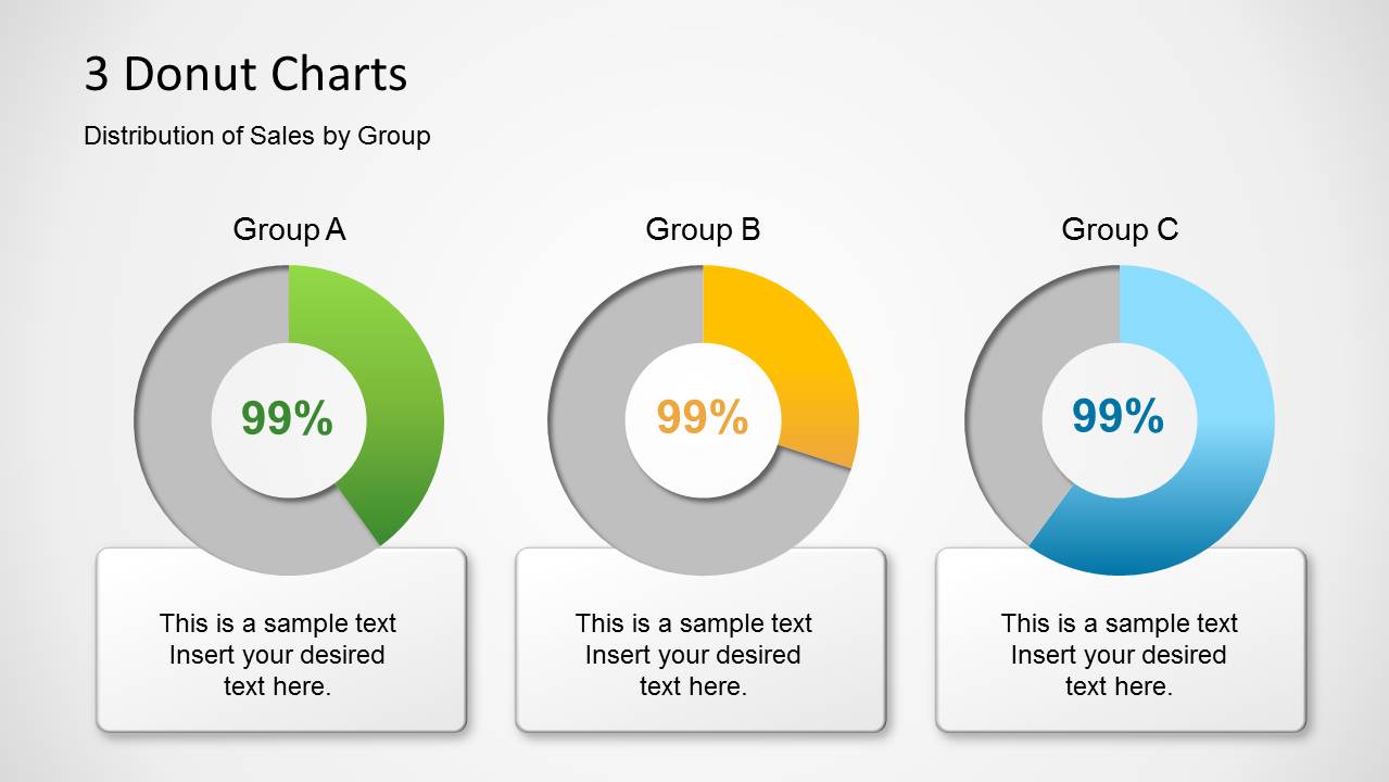
Donut Chart Template for PowerPoint - SlideModel

Custom data labels in a chart - Get Digital Help 21 Jan 2020 — Press with right mouse button on on any data series displayed in the chart. · Press with mouse on "Add Data Labels". · Press with mouse on Add ...

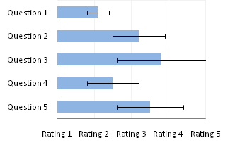
Text Labels on a Horizontal Bar Chart in Excel - Peltier Tech Blog

How to Make a Bar Chart in Excel - Smartsheet 25 Jan 2018 — Data labels show the value associated with the bars in the chart. This information can be useful if the values are close in range. To add data ...

30 How To Label Bar Graph In Excel - Labels Database 2020

How to Create Bar Chart in Excel? - EDUCBA Step 1: Select the data > Go to Insert > Bar Chart > Cone Chart. Step 2: Click on the CONE chart, and it will insert the basic chart for you. Step 3: Now, we need to modify the chart by changing its default settings. Remove gridlines of the above Chart. Change the chart title to Sales by month.